Plotting Camera Derived Snow Depths

Goal: Plot all camera location with pit locations. Then plot a timeseries of one camera in the trees and one in the open.

Approach:

1. Grab all the Site data for the pits and all the camera locations

2. Plot the pits and sites all together

3. Grab and Plot the Vegetated and Open Camera sites

Process

Step 1: Grab all the pit and camera locations

from snowexsql.db import get_db
from snowexsql.data import PointData, SiteData
from snowexsql.conversions import query_to_geopandas

from datetime import date
import geopandas as gpd
import matplotlib.pyplot as plt
import pandas as pd

# Connect to the database
db_name = 'db.snowexdata.org/snowex'
engine, session = get_db(db_name, credentials='./credentials.json')

# Grab all the point data that was that was measured with a camera
qry = session.query(PointData)
qry = qry.filter(PointData.instrument == 'camera')
qry = qry.filter(PointData.site_name == 'Grand Mesa')
qry = qry.filter(PointData.utm_zone == 12)

# Convert it to a geopandas df
camera_depths = query_to_geopandas(qry, engine)

# Grab all the unique pits geometry objects (locations)
qry = session.query(SiteData.geom)
qry = qry.filter(SiteData.site_name == 'Grand Mesa')
qry = qry.filter(SiteData.date > date(2019, 10,1))
qry = qry.filter(SiteData.date < date(2021, 10,1))

qry = qry.distinct()
pits = query_to_geopandas(qry, engine)

# Print out how many of each that we found
print(f'Found {len(camera_depths["geom"].unique())} camera locations')
print(f'Found {len(pits.index)} pit site locations')

# End our database session to avoid hanging transactions
session.close()

Found 18 camera locations
Found 226 pit site locations

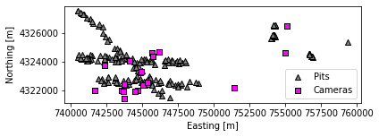
Step 2: Plot our camera and Pit locations

# plot our pits as triangles
ax = pits.plot(marker='^', color='gray', edgecolor='k', label='Pits')

# Plot our cameras as squares
ax = camera_depths.plot(ax=ax, color='magenta', edgecolor='k', marker='s', label='Cameras')

# Don't use scientific notation on the ticks for utm coords
ax.ticklabel_format(style='plain', useOffset=False)
ax.set_xlabel('Easting [m]')
ax.set_ylabel('Northing [m]')
ax.legend()
plt.tight_layout()
plt.show()

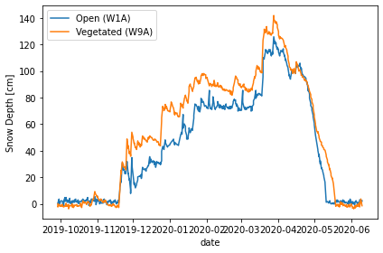
Step 3: Grab/Plot the Vegetated and Open Camera sites

# Grab the open site data from the db
open_site = 'W1A'
veg_site = 'W9A'
qry = session.query(PointData).filter(PointData.equipment.contains(open_site))
df_open = query_to_geopandas(qry,engine)

# Grab the vegetated site from the db
qry = session.query(PointData).filter(PointData.equipment.contains(veg_site))
df_veg = query_to_geopandas(qry,engine)

# Set the date as the index for easy plotting/reading
df_open = df_open.set_index('date')
df_veg = df_veg.set_index('date')

# Plot the 2 datasets by date!
ax = df_open['value'].plot(label=f'Open ({open_site})')
df_veg['value'].plot(ax=ax, label=f'Vegetated ({veg_site})')

# Mess with some labeling to make it look nice
ax.legend()
ax.set_ylabel('Snow Depth [cm]')
plt.tight_layout()
plt.show()

session.close()